Remedial ( Simple applications of tools of Demand and Supply)

Date 29.5.2020

We now take a look at the simple applications of Tools of Demand and Supply.

There are two types of government inteventions 
1.Price Ceiling: refers to fixing the maximum price of a commodity at a level lower than the equilibrium price.
Let us understand it by considering the commodity wheat and its price determination.
In the diagrm , demand curve DD and supply curve SS  of wheat intersect each other at point E  and as a result , Equilibrium price of OP  is determined.

Suppose , the equilibrium price OP  is very high and many poor people are unable to afford wheat at that Price .

Please go through the video link carefully to understand the topic better

https://www.youtube.com/watch?v=oDaa-voYNVQ

 2. PRICE FLOOR OR MINIMUM SUPPORT PRICE

Please go through the video link to understand the topic better

https://www.youtube.com/watch?v=eIPifiaGGiw

Remedial ( Main Market Forms)

Date : 29.5.2020

A very good morning boys 

Today we will be doing the main market forms.

Market refers to the whole region where buyers and sellers of a commodity are in contact with each otherto effect purchase and sale of a commodity.


There are two main forms of Market Structure
1. PERFECT COMPETITION
2. IMPERFECT COMPETITION :
The Imperfect Competition market form is divided into three parts

• Monopoly
• Monopolistic Competition
• Oligopoly

PERFECT COMPETITION: Perfect Competition refers to a market situation where there are very large number of buyers and sellers dealing in a homogeneous product at a price fixed by the market.

In a Perfectly Competitive market, sellers sell a homogeneous product at a single uniform price.This Price is not determined by a particular firm but by the Industry.

In reality, perfectly competition has never existed.

Features of Perfect Competition 

1. Very Large Number of Buyers and Sellers : There are a very  large number of buyers and sellers.

Implication: Very Large number of buyers and sellers is that the number of sellers is so large that the share of each seller is insignificant in the Total supply.It is the same case with demand with the buyers.

2. Homogeneous Product : The product for sale is identical in all respects like shape, size,quality, color,etc.

Implication: No individual firm is in aposition to charge a higher price for a product as the products are identical in all respects.

3. Freedom of entry and Exit: Every seller has the freedom to enter and exit the Industry.There are no artificial natural  barriers for entryof new firms and exit of existing firms.It  ensures absence of abnormal profits and abnormal losses in the long run.

Implication: Firms will only earn normal profits in the long Run.

UNDER PERFECT COMPETITION DEMAND CURVE IS A HORIZONTAL STRAIGHT LINE PARALLEL TO THE "X" AXIS

MONOPOLY:  refers to a market situation where there is a single  seller selling a product which has no close substitutes. Ex  Railways in India

Features of Monopoly 

1. Single Seller : Monopolist has full control over the supply and price of the product.No single buyer can influence can influence the market price.

2. No close substitutes: Thus, he has no fear of competition from new or existing products.

3. Restriction on Entry and Exit: As a result it earns (abnormal profits/abnormal losses) in the long runlong run  .

4. Price Discrimination: Charging different prices for the same product.

UNDER MONOPOLY THE DEMAND CURVE IS SLOPING DOWNWARD

Monopolistic Competition: refers to a market situation in which there are large number of firms which sell closely related but differentiated goods.Ex- Soaps, Toothpaste, etc

Features of Monopolistic Competition:

1. Large number of Sellers: Large number of firms selling closely related, but not homogeneous products.

2. Product Differentiation: refers to differentiating the product on the basis of brand, size, colour,etc.

3. Selling Cost: refers to expenses incurred on marketing, sales promotion and advertisment of the product.

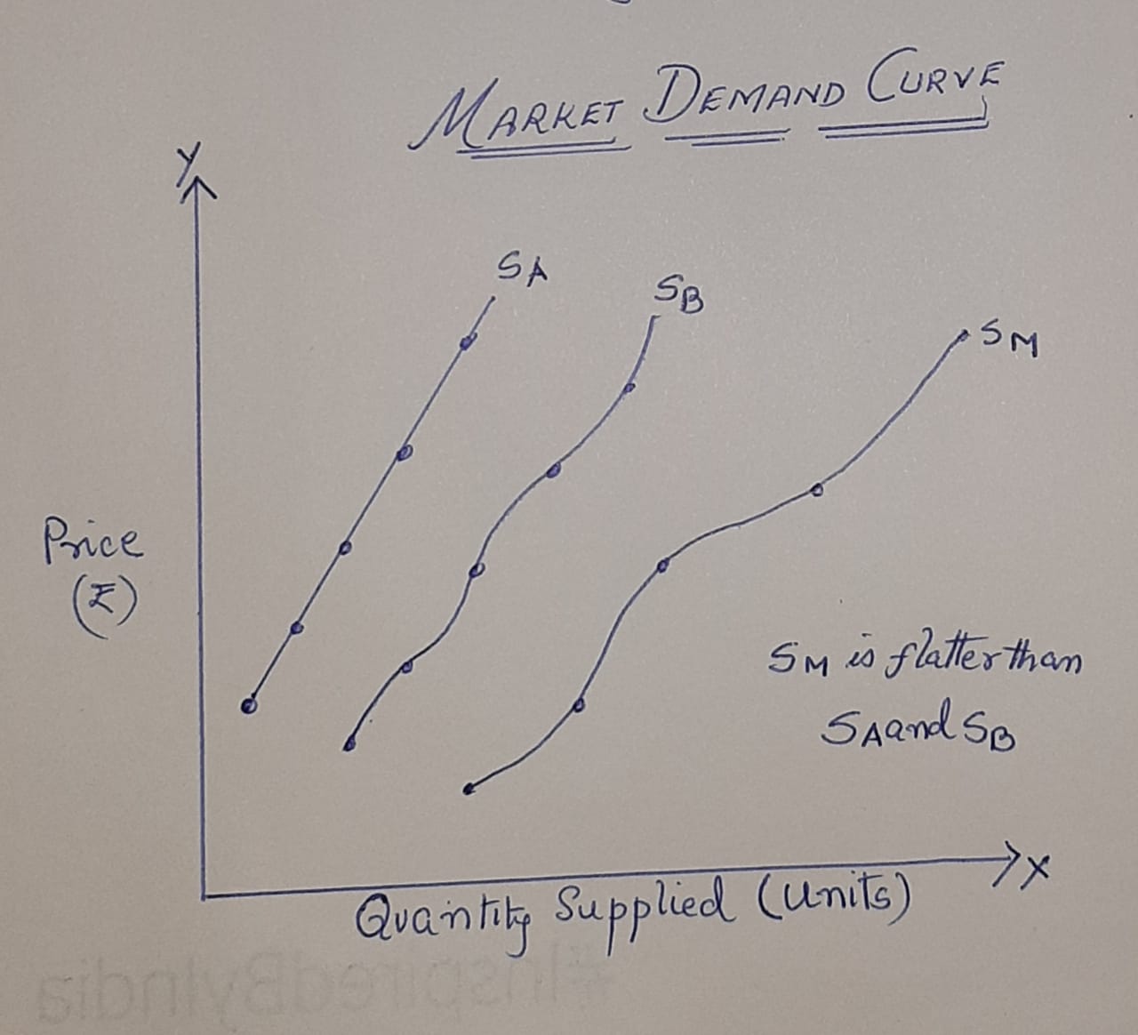
UNDER MONOPOLISTIC COMPETITION THE DEMAND CURVE IS DOWNWARD SLOPING WITH THE ONLY DIFFERENCE THAT IT IS MORE FLATTER THAN THE DEMAND CURVE OF MONOPOLY MARKET.

Oligopoly: refers to a market situation in which there are few firms selling homogeneous or differentiated products.

It is also known as competition among the few

Features of oligopoly

1. Few Firms : There are a few large firms.Exact number is not defined.Each producer produces a significant portion of the total output.Ex- automobiles 

2. Interdependence: Each firm is mutually dependent on the decision of its rival firm regarding price and output decision.

3. Non Price Competition: The firms dont practise Price discrimination but practise non price discrimination such as free insurance for a year, free gifts,etc

Dear boys i have put 4 videos for each market form respectively.

Make sure you watch them carefully to understand the topics better

https://www.youtube.com/watch?v=vqSVcCzZVbA

https://www.youtube.com/watch?v=7n9kFkytElU

https://www.youtube.com/watch?v=KRi_kK8XzHI

https://www.youtube.com/watch?v=J9zwhcoOFA8

Remedial(Cost)

Date: 28.5.2020

A very good morning students

Today we move to the next chapter which is cost.

Let us first understand a few important terms



COST: Cost in economics includes actual expenditure on inputs ( explicit cost) and the imputed value of the inputs supplied by the owners(implicit cos
Explicit Cost : It is the actual money expenditure on inputs or payment made to outsiders for hiring their factor services.Ex- Wages paid to employees

Implicit Cost : It is the cost of the self supplied factor of production.Ex- Slary for the service of entrepreneur

Thus, we can say that COST= Explicit Cost+ Implicit Cost


Cost Function : The relation between cost and output is known as 'Cost Function'
It refers to the functional relationship between cost and output
It is expressedas C = f(q)


Oppurtunity Cost : Oppurtunity Cost is the cost of the next best alternative forgone.


Short Run Cost: We know , in Short Run , some factors which are fixed, while others are variable.
Similarly, short run cost are also divided into two kinds of cost: Fixed Cost and Variable Cost
Sum of Fixed Cost and Variable Cost equals Total Cost


TOTAL FIXED COST(TFC) OR FIXED COST(FC) : Fixed Cost refers to those costs which do not vary directly with the level of Output. Ex- Rent of building,salary of permanent staff,etc
These are cost that cannot be changed in the short run

TOTAL VARIABLE COST(TVC) OR VARIABLE COST(VC): Variable cost refer to those costs whichvary directly with the level of output. Ex- payment of raw material,power,fuel,etc.
Such costs are incurred till there is productionand become zero at zero level of output.

TOTAL COST(TC) : Total Cost is the total expenditure incurred by a firm on the factors of production required for the production of a commodity.
                                             TC= TFC+TVC
Since TFC remains same at all levels of output, the change in TC is entirely due to TVC

Relationship between TC,TFC and TVC

• TFC curve is a horizontal straight line parallel to X-axis as it remains constant at all levels of output.
• TC and TVC curves are inversely S-shaped because they rise initially at a decreasing rate, then at a constant rate and finally,at an increasing rate.
• At zero output,TC is equal to TFC because there is no variable cost at zero level of output.So, TC and TFC  curves start from the same point, which is above the origin.
• The vertical distance between TFC curve and TC curve is equal to TVC.As TVC rises with increase in the output, the distance between TFC and TC curve also goes on increasing.
• TC nd TVC curves are parallel to each other and the vertical distance between them remains the same at all levels of output because the gap between them represents TFC,which remains constant at all levels of output.

AVERAGE COST:

Average Fixed Cost (AFC): Average fixed cost refers to the per unit fixed cost of  production.
                                        AFC = TFC/ Q ( Q= Quantity of Output)
AFC falls with increase in output as TFC remains same at all levels of output.
AFC is a rectangular Hyperbola,i.e. area under AFC curve remains same at different points.

AVERAGE VARIABLE COST (AVC) : Average variable cost refers to the per unit variable cost of production.
                                            AVC = TVC/Q  (Q= Quantity of Output) 
AVC initially falls with increase inoutput. Once the output rises till optimum level,AVC starts rising.It can be better understood with the help of a schedule and diagram given below.

AVERAGE TOTAL COST(ATC) or AVERAGE COST(AC)
Average cost refers to the per unit total cost of production.
                               AC = TC/Q        (Q= Quantity of Output)
Average cost is also defined as the sum of AFC+ AVC
Like AVC, average cost also initially falls with increase in output. Once the output rises till optimum level, AC starts rising. It can be better understood with the help of a schedule and diagram.

MARGINAL COST (MC) : Marginal cost refers to addition to Total Cost when one more unit of output is produced.
                                            MCn= TCn - TCn-1
                                                         OR
                                             MC = Change in TC/ Change in units of output
MC IS NOT AFFECTED BY FIXED COST 

The reason behind the 'U' shape of MC is the LAW OF VARIABLE PROPORTION.


Relation between AC and MC

• When MC is less than AC, AC fallswith increase in output
• When MC= AC, MC and AC intersecteach other.
• When MC is more than AC, AC rises with increase in output

AC depends on the nature of MC

• When MC curve lies below the AC curve, it pulls the latter downwards
• When MC lies above AC curve , it pulls the latter upwards
• Consequently, MC and AC are equal where MC intersect AC curve

Relationship between AVC and MC

• MC< AVC, AVC falls with increase in output
• MC = AVC , MC and AVC curves intersect each other
• MC> AVC, AVC rises with increase in output.

Relationship between AC and AVC

• AC is greater than AVC by the amount of AFC.
• The vertical distance between AC and AVC curves continues to fall with increase in output because the gap between them is AFC, which continues to decline with rise in output.
• AC and AVC curves never intersect each other as AFC can never be zero
• Both AC and AVC  curves are 'U' shaped due to the law of variable proportion
• MC curve intersects AVC and AC curves at their minimum points
• The minimum point of AC curve  lie always to the right of the minimum point of AVC curve.

Please go through the video links to understand the chapter better

https://www.youtube.com/watch?v=xZ6-h9Ib2LE

https://www.youtube.com/watch?v=Yr0eiVdK1RY

https://www.youtube.com/watch?v=uVFPB90gpWM&t=158s

Remedial (Revenue)

Date : 28.5.2020

Let us begin with the next topic Revenue

Revenue refers to the amount recieved by a firm from the sale of a given quantity of a commodity in the market.


CONCEPT OF REVENUE: The concept of Revenue consists of 3 important terms

1. Total Revenue : Total Revenue refers to the Total reciepts from the sale of a given quantity of a commodity.
TR = Quantity X Price.

2. Average Revenue : Average Revenue refers to the revenue per unit of output sold.
 AR = TR/QUANTITY
 AR is also equal to the Price

3. Marginal Revenue : Marginal Revenue is the additional revenue generated from sale of an additional unit of output.
   MR = TRn - TRn-1     Or        MR= Change in TR/ Change in number of units

TR is the summation of MR
The concept of TR, AR and MR can be better understood from the table given below

Relationship between Revenue Concepts: It can be discussed under two situations
1. When Price remains constant: It means, any quantity of a commodity can be sold at a particular Price.

2. When Price Falls with rise in Output : Sales can be increased only by lowering the Price.



Relationship between AR and MR when Price is constant: Always remember that when a firm is able to sell more output at the same price, then AR =MR at all levels of output.

Relationship between TR and MR when Price is constant: MR and AR curves are horizontal straight lines parallel to X axis . Since MR remains constant, TR also increasesat a constant rate.Due to this reason , the TR curve is positively sloped straight line. As TR is zero at zero level of output , the TR curve starts from the origin.

Relationhsip between AR and MR  ( When Price falls with rise in output) : When firms can increase their volume of sales only by decreasing the price, then AR falls with increase in sales.It means , revenue from every additional unit (MR) will be less than AR. As aresult both AR and MR curve slopes downwards from left to right.
The relationship can be better understood through the schedule and graph.

General relationship between AR and MR

1. AR increases as long as MR is higher than AR
2. AR is maximum and constant when MR is equal to AR
3. AR falls when MR  is less than AR

Please go through the video links to understand the chapter better

https://www.youtube.com/watch?v=LJx7HW6E-8s

https://www.youtube.com/watch?v=VgtDXepSz7E

Remedial ( Producer's Equilibrium)

Date : 28.5.2020

We now shift our focus to the third topic for the day (Producer's Equilibrium) 

Before getting to the topic it is very important to understand that this chapter deals with determination of a level of output , which yields the maximum profit.

Profit: Profit refers to the excess of reciepts from the sale of goods over the expenditure incurred on producing them.


Producer's Equilibrium: Producer's Equilibrium refers to that price and output combination which brings maximum profit to the Producer and Profit as more is produced.


In class 12 we will be studying the Marginal Revenue and Marginal Cost Approach(MR-MC Approach)

The conditions needed for the Approach are 

• MR=MC
• MC is greater than MR after MC=MR output level

Producer's Equilibrium ( when Price remains constant)

Please go through the video link well to understand the topic better


https://www.youtube.com/watch?v=_2-XKkVFEls&t=717s



https://www.youtube.com/watch?v=wCead9i8XIs

Remedial (Production Function)

Date : 27.5.2020



A very good morning boys 

Today we begin with the chapter Production Function


Production Function is an expression of the technological relation between phusical inputs and output of a good.

A few important things you should know:

Short Run: Short Run refers to a period in which output can be changed by changing only variable factors.

Long Run: Long Run refers to a period in which output can be changed by changing all factors of production

Variable Factors : Variable Factors refer to those factors, which can be changed in the short run. Ex Raw material, power, etc

Fixed Factors : Fixed Factors refer to those factors, which cannot be changed in the short run. Ex Plant and Machinery, Building, etc

OUR SYLLABUS IS RESTRICTED TO SHORT RUN PRODUCTION FUNCTION also known as ( LAW OF VARIABLE PROPORTION)

CONCEPT OF PRODUCT: 
Total Product : refers to total quantity of goods produced by a firm during a given period of time with the given number of inputs.

Average Product : refers to output per unit of variable input.
AP= TP/Units of variable factor

Marginal Product : refers to addition to total product, when one more unit of variable factor is employed.
MP=TPn-TPn-1            OR   MP= Change in TP/ Change in units of variable factor

TP is the summation of MP



LAW OF VARIABLE PROPORTION

Law of Variable Proportion states that as we increase quantity of onlt one input keeping all other inputs fixed, TP initially increases at an increasing rate, then at a decreasing rate and finally at a negative rate.

Law of Variable Proportion is also known as "Law of Returns" or "Law of Returns to a Factor"

Assumptions of Law of Variable Proportions
1. Operates in short run, as factors are classified as variable and fixed factor
2. This Law applies to the field of production only
3. The state of technology is assumed to be constantduring the operation of this law.
4.It is assumed that all variable factors are equally efficient.

Let us now understand the law
Suppose a farmer has 1 acre of land (fixed factor) on which he wants to increase the production of wheat with the help of labour(variable factor).When he employed more and more units of labour, initially output increased at an increasing rate,then at a decreasing rate and finally at a negative rate.
This behaviour is shown through a table

Fixed Factor(Land in acres)	Variable Factor(Labour)	TP(Units)	MP(Units)	Phase
1	1	10	10	1st (increasing returns to a factor)
1	2	30	20
1	3	45	15	2nd (Diminishing Returns to a factor)
1	4	52	7
1	5	52
1	6	48	-4	3rd( Diminishing returns to a factor)

As seen in the above table and diagram

We see that there are three phases to the law of variable proportion.
Increasing Returns to a Factor, Decreasing Returns to a Factor and the Diminishing Returns to a Factor.



A rational producer will always seek to operate in the 2nd phase of the Law of Variable Proportion.
In 1st phase there is scope for more profit if production is increased with more units of variable factors.
In 3rd phase , MP  of each variable factor is negative.No rational producer would like to produce where he is getting negative returns.
So every rational producer will produce in the 2nd phase as in this phase Total Productivity is maximum and Marginal Productivity of each variable factor is positive.


Reson for Increasing Returns(1st Phase)
1. Better utilisation of Fixed Factors
2. Increased Efficiency of Variable factors
3. Indivisibility of Fixed Factors


Reason for Diminishing Returns to a Factor(2nd Phase)
1. Optimum combination of factors.
2. Imperfect Substitutes

Reason for Negative Returns to a Factor(3rd Phase)
1. Limitation of Fixed Factor
2. Poor coordination between variable and fixed factors
3. Decrease in Efficiency of Variable Factor


Relation between TP and MP
1. As long as TP increases at increasing rate ,MP also Increases
2. When, TP increases at diminishing rate, MP decreases
3. When TP reaches maximum point MP becomes zero.
4.When TP starts decreasing, MP becomes negative

Relationship between AP and MP
1. As long as MP is more than AP, AP rises
2. When MP is equal to AP, AP is at its maximum
3. When MP is less than AP, AP falls, but becomes negative. 

Please go through the 2 video links given below to understand the chapter very well


https://www.youtube.com/watch?v=eWJUFHkiulI


https://www.youtube.com/watch?v=UZaaTFmxwVg

Remedial (Supply)

Date : 26.5.2020

A very good morning boys

Let us now shift our focus to Supply

                1.Supply is always expressed with reference to price 
                2. Supply is always with respect to a period of time
                3. Supply is a desired quantity
                4. Supply of a commodity does not comprise the entire stock of the commodity

To sum up we can say Supply is the quantity of a commodity that a firm  is willing and able to sell,at each possible price during a given period of time.

Supply for a commodity may be either with respect to an individual or to the entire market.
1. Individual Supply : 
2. Market Supply:

Determinants of Supply ( Individual Supply)

1. Price of the given commodity : There exists an direct relation between Price and quantity supplied.

2.Price of Other Goods : Increase in price of other goods makes them more profitable in comparison to the given commodity.So, the supplier shifts his resources to the production of the other good.

3.Prices of Factors of Production (Inputs): There is an inverse relation between the prices of factors of production and supply                                                           

4. State of Tecnology: If there is upgraded technology supply of the product increases and vice-versa

5. Government Policy: If taxes increases the supply fall and vice-versa

6. Goals /Objectives of the firms : There are two objectives of a producer : 

• Profit maximisation
• Sales maximisation

Determinants of Market Supply
1.Number of firms in the market: More the number of firms in the market more will be the supply of products in the market and vice-versa

2. Future expectation regarding price: If the seller expects prices to fall in future he will try and sell more of the commodity in the present time and vice-versa

3. Means of Transportation and communication: Better means of Transportation and communication will increase the supply of the product and vice-versa

NOTE: All the above factors will be taken into consideration only by keeping all other factors constant.

Supply Function: It shows the relationship between quantity supplied for a particular commodity and the factors influencing it.
It means a relationship of quantity supplied for a particular commodity with any of the above factors mentioned

Supply Schedule : Is a tabular representation of various quantities of a commodity being supplied at various levels of price, during a given period of time.

                                                      Individual Supply Schedule

Price	Quantity supplied of a commodity X(in units
1	5
2	10
3	15
4	20
5	25

                                                    

                                                         Market Supply Schedule

Price	Individual Supply		Market Demand (in units ){SA + SB }
	Household  A (SA)	Household  B (SB)
1	5	10	5+10 = 15
2	10	20	10+20 =30
3	15	25	15+25= 40
5	20	35	20+35= 55
5	25	40	25+ 40= 65

Supply Curve : It is a graphical representation of Supply schedule.

Individual Supply Curve : It refers to a graphical representation of individual Supply schedule.

Market Supply Curve : refers to a graphical representation of market Supply schedule.

Market Supply curve is obtained by horizontal summation of the individual  supploycurves {S_A + S_B }

Market Supply Curve is Flatter : because as price changes, proportionate change in Market supply is more than proportionate change in individual supply.

Law of Supply : states the inverse  relationship between price and quantity supplied, keeping other factors constant ( ceteris paribus). 

Assumptions of Law of supply

1. Price of other goods do not change.

2. There is no change in the state of technology.

3. Prices of factors of production remains the same.

4. There is no change in the taxation policy.

5. Goals of the producer remain the same.

Price	Quantity supplied of a commodity X(in units
1	10
2	20
3	30
4	40
5	50

Movement along the Supply Curve VS  Shift in SupplyCurve

For Elasticity of Supply please refer to the text books